
Best OBV Calculation Tools in Julia to Buy in July 2026
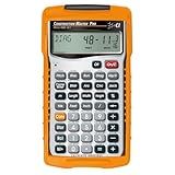
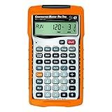
Calculated Industries 4065 Construction Master Pro Advanced Construction Math Feet-inch-Fraction Calculator for Contractors, Estimators, Builders, Framers, Remodelers, Renovators and Carpenters
-
QUICKLY SOLVE DIMENSIONAL MATH FOR ACCURATE BUILDING LAYOUTS.
-
EFFORTLESSLY CONVERT BETWEEN ALL COMMON DIMENSION FORMATS.
-
REDUCE MATERIAL WASTE WITH PRECISE ESTIMATING AND ADVANCED SOLUTIONS.


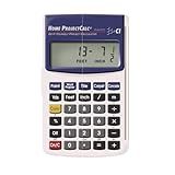
Calculated Industries 8510 Home ProjectCalc Do-It-Yourselfers Feet-Inch-Fraction Project Calculator | Dedicated Keys for Estimating Material Quantities and Costs for Home Handymen and DIYs , White Small
-
CONVERT MEASUREMENTS INSTANTLY BETWEEN IMPERIAL AND METRIC UNITS.
-
EASILY CALCULATE MATERIAL NEEDS TO AVOID SURPRISES AT CHECKOUT.
-
ESTIMATE EXACTLY THE PAINT AND TILES YOU NEED FOR YOUR PROJECTS.
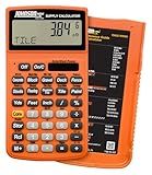
Johnson Level & Tools CALC-0000 Supply Calculator
- PRE-PROGRAMMED FUNCTIONS FOR QUICK TRADE CALCULATIONS.
- OVERSIZED LCD DISPLAY FOR EASY READABILITY ON SITE.
- RUGGED, SOLAR-POWERED DESIGN WITHSTANDS TOUGH ENVIRONMENTS.
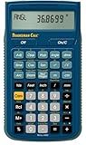
Calculated Industries 4400 TradesmanCalc Technical Trades Dimensional Trigonometry and Geometry Math and Conversion Calculator Tool for Tech Students, Welders, Metal Fabricators, Engineers, Draftsmen Small
-
EASILY SOLVE ALL FRACTIONS IN MULTIPLE FORMATS FOR PRECISE CALCULATIONS.
-
CONVERT BETWEEN IMPERIAL AND METRIC UNITS FOR STRAIGHTFORWARD MATH.
-
CUT COSTS AND WASTE WITH BUILT-IN SOLUTIONS FOR CRITICAL MEASUREMENTS.
Calculated Industries 4080 Construction Master Pro Trig Advanced Construction Math Feet-Inch-Fraction Calculator with Full Trig Function for Architects, Engineers, Contractors, Estimators and Framers
- SOLVE DIMENSIONAL MATH ACCURATELY AND QUICKLY WITH EASE!
- EFFORTLESSLY CONVERT ALL COMMON BUILDING DIMENSION FORMATS!
- SAVE TIME, REDUCE WASTE, AND AVOID COSTLY ERRORS ON PROJECTS!
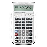
Calculated Industries 8030 ConversionCalc Plus Ultimate Professional Conversion Calculator Tool for Health Care Workers, Scientists, Pharmacists, Nutritionists, Lab Techs, Engineers and Importers
-
CONVERT 70+ UNITS EASILY: ENTER MEASUREMENTS LIKE YOU SAY THEM!
-
500+ COMBINATIONS: NO COMPLEX CALCULATORS OR FORMULAS NEEDED!
-
BOOST ACCURACY & SAVE TIME: SIMPLIFY CONVERSIONS AND CALCULATIONS DAILY!
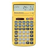
Calculated Industries 4019 Material Estimator Calculator | Finds Project Building Material Costs for DIY’s, Contractors, Tradesmen, Handymen and Construction Estimating Professionals,Yellow
- CUSTOMIZABLE MEASUREMENTS: ENTER DIMENSIONS IN VARIOUS FORMATS EFFORTLESSLY.
- MATERIAL ESTIMATION: QUICKLY DEFINE AND ESTIMATE PROJECT MATERIAL NEEDS.
- BUILT-IN CALCULATORS: INSTANTLY CALCULATE QUANTITIES TO AVOID COSTLY ERRORS.
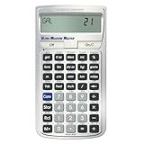
Calculated Industries 8025 Ultra Measure Master Professional Grade U.S. Standard to Metric Conversion Calculator Tool for Engineers, Architects, Builders, Scientists and Students | 60+ Units Built-in, Silver
- OVER 400 CONVERSION COMBOS FOR EFFORTLESS MEASUREMENTS AND ACCURACY!
- USER-FRIENDLY DESIGN: INPUT DATA AS YOU SPEAK FOR QUICK RESULTS!
- SAVES TIME AND REDUCES ERRORS-AN INVALUABLE TOOL FOR DAILY TASKS!
Calculated Industries 4020 Measure Master Pro Feet-Inch-Fraction and Metric Construction Math Calculator, Silver
- EFFORTLESSLY CONVERT U.S. IMPERIAL AND METRIC MEASUREMENTS WITH EASE.
- SIMPLIFY JOBSITE CALCULATIONS FOR ACCURATE MATERIAL NEEDS AND COST ESTIMATES.
- BUILT-IN CIRCULAR MATH FOR PRECISE LAYOUTS-NO FORMULAS NEEDED!
Calculated Industries 8528 Metric Do-It-Yourself Calculator Small
- METRIC-FRIENDLY: WORK IN CM/METRES FOR PRECISION ACROSS PROJECTS.
- BTU CALCULATOR: EASILY CONVERT AND CALCULATE HEATING REQUIREMENTS.
- CUSTOMIZABLE DEFAULTS: TAILOR METRIC VALUES TO FIT ANY PROJECT NEED.
On-Balance Volume (OBV) is a technical analysis tool used to track the flow of volume in and out of a security. It is calculated by adding the volume on days when the price closes higher than the previous day's close, and subtracting the volume on days when the price closes lower than the previous day's close.
In Julia, you can compute the OBV for a given security by first importing the necessary packages such as DataFrames and Plots. Next, you can create a function that takes in the price data and volume data for the security, and calculates the OBV values based on the rules mentioned above.
You can then visualize the OBV values using a plot to identify any trends or patterns in the volume flow of the security. This can help traders and investors make more informed decisions about when to buy or sell a security based on the volume dynamics.
How to calculate OBV divergence in Julia?
To calculate On-Balance Volume (OBV) divergence in Julia, you can follow these steps:
- First, you need to calculate the OBV values based on the price and volume data. This can be done using the following formula:
OBV[i] = OBV[i-1] + sign(close[i] - close[i-1]) * volume[i]
Where:
- OBV[i] is the OBV value at index i
- OBV[i-1] is the OBV value at the previous index
- sign() is a function that returns -1 if the argument is negative, 0 if it is zero, and 1 if it is positive
- close[i] is the closing price at index i
- volume[i] is the volume at index i
- Next, you can calculate the OBV divergence by comparing the OBV values with the price values. If the OBV values are moving in the opposite direction of the price, then it is considered a divergence. You can calculate the OBV divergence by subtracting the current OBV value from the previous OBV value.
- You can then plot the OBV divergence to visualize the divergence and identify potential trend reversals.
Here's a sample code snippet in Julia to calculate OBV divergence:
using DataFrames
function calculate_OBV_divergence(close::Vector{Float64}, volume::Vector{Float64}) OBV = zeros(length(close)) OBV[1] = volume[1]
for i in 2:length(close)
    if close\[i\] > close\[i-1\]
        OBV\[i\] = OBV\[i-1\] + volume\[i\]
    elseif close\[i\] < close\[i-1\]
        OBV\[i\] = OBV\[i-1\] - volume\[i\]
    else
        OBV\[i\] = OBV\[i-1\]
    end
end

OBV\_divergence = OBV\[2:end\] - OBV\[1:end-1\]

return OBV\_divergence
end
Sample price and volume data
close = [10.0, 11.0, 12.0, 11.5, 11.0] volume = [1000.0, 1500.0, 2000.0, 1800.0, 1200.0]
OBV_divergence = calculate_OBV_divergence(close, volume)
Plot the OBV divergence
using Plots plot(2:length(close), OBV_divergence, xlabel="Index", ylabel="OBV Divergence")
This code snippet defines a function calculate_OBV_divergence that calculates the OBV values and then calculates the OBV divergence based on the price and volume data. It then plots the OBV divergence to visualize the divergence.
You can modify the code as needed to suit your specific requirements and data format.
How to calculate OBV trendlines in Julia?
One way to calculate On-Balance Volume (OBV) trendlines in Julia is to first calculate the OBV values and then fit a trendline to those values using a regression model. Here is an example of how to do this in Julia:
using DataFrames using GLM
Sample data
volume = [100, 150, 200, 250, 300, 200, 150, 100, 50, 0] close = [10, 12, 14, 16, 18, 15, 12, 9, 6, 3]
Calculate OBV values
obv = zeros(length(close)) obv[1] = 0 # initial OBV value for i in 2:length(close) if close[i] > close[i-1] obv[i] = obv[i-1] + volume[i] elseif close[i] < close[i-1] obv[i] = obv[i-1] - volume[i] else obv[i] = obv[i-1] end end
Fit a linear trendline to OBV values
df = DataFrame(obv = obv) model = lm(@formula(obv ~ 1:length(close)), df) trendline = predict(model)
Plot the OBV values and trendline
using Plots plot(close, label="Close Price", xlabel="Day", ylabel="Price") plot!(obv, label="OBV Values", xlabel="Day", ylabel="Volume") plot!(trendline, label="Trendline")
This code snippet calculates OBV values for a given set of volume and closing prices, fits a linear trendline to the OBV values using a simple linear regression model from the GLM package, and then plots the closing prices, OBV values, and the trendline. You can customize this code to fit other types of trendlines (e.g., polynomial, exponential) if needed.
How to plot OBV in Julia?
To plot On-Balance Volume (OBV) in Julia, you can use the Plots.jl package. Here is an example code snippet to plot OBV using Plots.jl:
using Plots
Sample data for OBV
close_prices = [100, 105, 110, 115, 120, 115, 110, 105, 100] volume = [5000, 6000, 7000, 8000, 9000, 8000, 7000, 6000, 5000]
Calculate OBV
obv = cumsum(volume .* sign(diff(close_prices)))
Plot OBV
plot(obv, xlabel="Date", ylabel="OBV", label="OBV", legend=:bottomright)
This code snippet creates a plot of OBV using sample data for close prices and volume. You can replace the sample data with your own data to visualize the OBV for different stocks or assets. Make sure to install the Plots.jl package before running this code by using the following command:
using Pkg Pkg.add("Plots")